Page 62 - Spring2020

Arctic Acoustic Oceanography
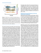
Figure 11. Travel times as a function of yearday (yearday 1 is defined to be January 1, 2016. The yeardays continue into 2017 for transmissions from mooring T5 to mooring T6 during the 2016–2017 CANAPE experiment (see Figure 10). The range is approximately 149 kilometers. Each peak in the acoustic receptions that exceeds a specified threshold is plotted as a dot. The size of the dots is proportional to the signal-to-noise ratio, and the color indicates the vertical arrival angle at the receiver. See text for a further explanation.
The acoustic transceivers were similar to those used in Fram Strait. Each source transmitted every four hours. The resulting arrival structures can be conveniently summarized in “dot plots” constructed for each source-receiver pair in which the travel times of the peaks in each reception are plotted versus yearday (Munk et al., 1995). The receptions at mooring T6 (in the center of the array) for transmissions from mooring T5 are shown in Figure 11. There are multiple ray paths along which the trans- mitted signal travels from the source to the receiver (eigenrays). Each approximately horizontal line in the plot corresponds to arrivals from a specific ray path. For example, the arrivals at ~102.2 seconds are from a ray path that has a lower turning depth close to 2,000 meters. The color indicates that the vertical arrival angle at the receiver is about +12° (traveling upward). The closely spaced arrivals between approximately 102.6 and 103.4 seconds have much shallower lower turning depths and interact more frequently with the surface than the deeper turning rays. The disappearance of the arrivals clearly shows the effects of the increased losses that occur as the ice cover reaches a maximum thickness of about 1.5 meters in late winter. The unresolved, low-angle arrivals occurring after about 103.4 seconds are from energy largely trapped in the Beaufort Duct.
The dot plots show that that the measured travel times are remarkably stable, with peak-to-peak variability of only about 20 milliseconds over the entire year. In comparison, travel times in midlatitudes at similar ranges vary by something like an order of magnitude more (~200 milliseconds peak to peak) due to the effects of ocean mesoscale variability, with spatial scales of roughly 100 kilometers and timescales of about 1 month.
Multipurpose Acoustic Systems in the Arctic Ocean Observing System
Monitoring and understanding the rapid changes underway in the Arctic Ocean are of crucial importance in assessing its role in climate variability and change. In addition, as the
Arctic converts from a largely perennial ice cover to a sea- sonal ice cover, oil and gas exploration, fisheries, mineral extraction, shipping, and tourism will increase the pressure on the vulnerable Arctic environment, requiring improved ocean-ice-atmosphere data to inform and enable sustainable development while protecting this fragile environment.
Multipurpose acoustic systems can make important contribu- tions to an integrated Arctic Ocean observing system designed to observe the rapid changes underway in the Arctic, taking advantage of the fact that acoustic signals can travel long dis- tances beneath the ice (Mikhalevsky et al., 2015; Howe et al., 2019). Acoustic networks can provide under-ice navigation for floats, gliders, and autonomous underwater vehicles. They can measure large-scale temperatures and currents (ocean acoustic tomography). Passive acoustic monitoring of natural sounds can provide information on marine life, ice, and seis- mic events, whereas monitoring of anthropogenic sounds can help assess the potential for impacts on marine animals. In an integrated multipurpose acoustic system, the same sources generate signals for both underwater navigation and ocean acoustic tomography. The receivers used for ocean acoustic tomography are also used for passive acoustic monitoring. The spatially averaged temperature fields provided with high temporal resolution by ocean acoustic tomography and the high spatial resolution data provided by floats, gliders, and autonomous underwater vehicles are naturally complemen- tary. Both data types provide constraints for ocean general circulation models. Pilot multipurpose acoustic networks were successfully implemented on a regional scale in the 2010–2012 ACOBAR and 2014–2016 UNDER-ICE projects
62 | Acoustics Today | Spring 2020