Page 13 - Winter 2020

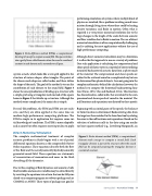
Figure 2. Finite-difference method (FDM), a computational discrete grid concept to compute a sound field. The space is broken into a grid of boxes called elements where the sound is considered constant in each element and is summed over all space.
up into a mesh, which looks like a wire grid applied to the structure of various shapes, often triangles. The points of the chosen mesh shape are called nodes, and these define the shape of the mesh. The goal of the method is to sum the contribution of each element to the sound field. Figure 3 shows the conceptualization of dividing up a structure with a simple grid using a triangular mesh instead of the square boxes in Figure 2 that divide up a structure. Although the method seems complicated, the main idea is simple.
For real-life problems, the FDM and FEM are not exclu- sive, and they are often applied at the same time on modern high-performance computing platforms. The FDM is simple in its application but requires some ini- tial knowledge of conditions. The FEM is more adaptable and accurate but often requires more input data to apply.
Direct Numerical Simulation
The complete mathematical treatment of complex acoustic problems in fluids begins with a set of partial differential equations known as the compressible Navier- Stokes equations. These equations describe both the flow of the fluid and the aerodynamically/hydrodynamically generated sound field. These equations are statements of conservation of momentum and mass in the fluid, describing all the dynamics.
Due to this coupling of fluid dynamics and acoustics, both fluid variables and acoustic variables may be solved directly by rewriting the equations into a form that can be fully sim- ulated via a computer program or software package such as COMSOL or ANSYS. These types of packages are good at
performing simulations of systems where multiple kinds of physics are involved, like a problem involving sound trans- mission through living tissue where there could be heating, density variations, and fluids in motion. Often what is required is a very precise numerical resolution due to the large changes in the length of the scales between acoustic and flow variables due to fluids in motion. The use of direct numerical simulation is often computationally challenging and is unfitting for most applications without the use of high-performance computing.
Although direct numerical simulation may be a limitation, it is often the first approach to use on a variety of problems. One such application is calculating the compressional and shear speeds of elastic waves in a material of interest utilizing measured backscattered acoustic data from a sphere made of the material. The compressional and shear speeds are related to the scattered sound in a complicated way but can be determined for spherical objects. I am not going into the complex mathematics behind the calculations; however, the method is to compute the theoretical backscattering func- tion (Faran, 1951; Chu and Eastland, 2014). This function has discontinuities, called nulls, that are related to the com- pressional and shear speeds of sound in the material. The null locations and separations are dictated by these speeds.
Beginning with an initial guess of the speeds, the backscat- ter form function is determined. Backscattering data from the target are then matched to the form function by relating the error in the null locations and separations. Based on the selection of arbitrary nulls in the data using any nonlin- ear least squares method (e.g., Levenberg-Marquardt), an
Figure 3. Finite-element method (FEM), a computational element mesh concept to compute a sound field. Each triangular division is part of the structure where the sound field can be computed assuming the triangular division is considered constant.
Spring 2021 • Acoustics Today 13