Page 15 - Winter 2020

and receiver positions cannot be justified by utilizing the theoretical solution of the wave equation.
An example application of an integral method is to calculate the acoustic field from a hexagonal array of sources treated as point sources. Figure 5a shows an example of an array of 31 sources arranged as a grouping of hexagons. The loca- tions are determined computationally, with each node being treated as an acoustic point source. The field is summed over all sources, and the level is calculated at a given range. This could be done over time to create a movie of the acoustic field that can provide insight into how the acoustic wave propagates. The simulation is assumed to be underwater with a source frequency of 10 kHz. An example might be a source array, but the problem is easily simulated using inte- gral methods. The array used in Figure 5a has the output given as a color plot in Figure 5b, respectively.
Kirchhoff Integral
Kirchhoff and Helmholtz were able to show that sound radiating from a localized source in a limited area can be described by enclosing this source area by an arbitrarily envisioned surface. The sound field inside or outside the chosen surface is calculated using the Helmholtz equa- tion. The solution can be determined by the sum of a set of “basis” functions related to the geometry of the problem that can be used. The difficulty in the problem is determin- ing the functions that work and is not described here due to being out of scope of this article. The calculated field on the surface directly follows from the wave equation.
A variation of the scheme allows one to calculate the pres- sure on the arbitrary surface using the normal particle velocity, which is the mechanism involved in acoustic trans- mission. The particle velocity perpendicular to the surface could be given by a FEM simulation of a moving structure. However, the modification of the method to avoid utilizing the acoustic pressure directly on the surface leads to snags, with enclosed volumes being driven at their resonant fre- quencies. This is a major issue in the implementation of the technique. To get around this limitation, the sound pressure is determined on the surface of the object first and then imaginary sources are added on its surface to cancel the normal particle velocity on the surface of the object.
An instance of the use of the Kirchhoff integral is to divide the physical domain into a smaller simpler set of parts for a more complex problem, which introduces the
application of the FEM (Everstine and Henderson, 1990). This is another example of integral methods, but it solves the field by direct integration over the surface. The goal is to split the computational area into different regions so that the central acoustic equations can be solved with
different sets of equations and numerical techniques.
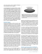
For instance, simulating an idealized Helmholtz resona- tor (such as a violin or guitar) as a flower vase and solving the wave equation with boundary conditions becomes difficult due to the odd shape of the boundary. To solve this, therefore, the boundary is broken up into smaller pieces, and the acoustic field is calculated for each indi- vidual piece of the boundary. A concept figure showing what the boundary would look like is shown in Figure 6.
The method would then employ breaking up the vase into physical elements, as in Figure 3, where all the corners of the element are broken into nodes. The method just sums the acoustic field from each individual element for each node in space, assuming some constant coefficient given as
for each element, approximated from the boundary and field equations. Each element would be given as some shape function given as , which was a triangle in Figure 3. The total acoustic field is determined as a sum of each individual
Figure 6. Possible spatial division, called discretization, of a Helmholtz resonator in the form of a vase. Each rectangle is treated as an individual point where the sound field is considered constant.
contribution such as p(x,y,z)≈
are the obligatory spatial variables.
Machine Learning and Other Contributions
Several significant contributions have been made in dif- ferent areas of investigation with the applications of computational acoustics. One of these is the incorporation
=1
,
,wherex,y,andz
Spring 2021 • Acoustics Today 15