Page 14 - Winter 2020

COMPUTATIONAL ACOUSTICS METHODS
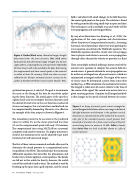
Figure 4. Dashed black curve, theoretical target strength determined from the form function; blue solid curve, backscattered data-determined target strength of a 64-mm copper sphere, comparing theory and experiment; red circles, the three chosen nulls to be matched to the data, determining the compressional and shear sound speeds in the material to within at least 6% accuracy. Work was done on sonar calibration for biomass estimated acoustic surveys by the author at Northwest Fisheries Science Center (Seattle, WA).
optimization process is selected. The goal is to minimize the error in the fitting of the data by iteratively updat- ing the form function. The initial guess of the speeds is updated and used to recompute the form function until the desired level of error in the cost function is achieved.
As one can imagine, this is a brute force method and can be computationally demanding. However, it is effective.
An example of the data output is shown in Figure 4.
The simulation proved to be accurate in the predicted values to within 6% on the shear speed and less than 5% on the compressional speed with only 22 iterations. The computational time using MATLAB on a personal computer took nearly 10 minutes. If a higher precision is desired, the minimum error can be adjusted to get more iterations but will take much longer.
The first of these various numerical methods often used to determine the sound pressure in a computational acous- tics problem is the FDM. The method takes the continuous differential equation that describes the phenomena and breaks it in to a finite algebraic set of equations. The details are left out in this article for brevity; however, the useful- ness of this method is hard to deny. The method is used by breaking up the space into a grid of points, and the sound
field is calculated with small changes in the field based on the nearest grid points in the space. The solution is found by solving numerically using small steps in space and time. This technique is used in multiple areas and works well for wave propagation and scattering problems.
By way of an illustration (see Bunting et. al., 2020), the application of the wave equation and discretization shows the power of computational acoustics. Assuming harmonic time dependence of pressure and applying the wave equation, one obtains the Helmholtz equation. The Helmholtz equation describes steady-state wave propaga- tion in physics and relates to acoustic wave propagation through either the particle velocity or pressure in a fluid.
There are multiple methods utilizing a known result of the acoustic wave equation to compute the acoustic field of a sound source. A general solution for wave propagation can be written as an integral over all present sources, which are summarized as integral methods. The origin of the acous- tic source must be determined a priori from some other method (e.g., a FEM simulation of a mechanical structure). The integral is taken over all sources relative to the time of the source of the signal. The sound wave arrives later at a given receiving position. Common to all integral methods is that changes in the speed of sound between the source
Figure 5. a: Array of acoustic point sources arranged as several hexagonal distribution where cross-range is the lateral left/right dimension and elevation is the up/down vertical dimension as a demonstration of the method. b: An acoustic color plot of the simulated acoustic sound pressure level measured at a location 10 m from a source array of 31 point sources being driven in unison at 10 kHz. Yellow is louder than darker blue to a level in decibels relative to 1 μPa of acoustic pressure.
14 Acoustics Today • Spring 2021