Page 56 - Winter 2020

UNDERWATER GPS
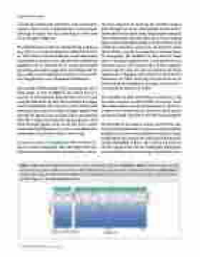
a sound speed minimum referred to as the sound chan- nel axis, which exists at approximately 1,000 m depth, although the depth can vary depending on where you are on the globe (Figure 3).
The SOFAR channel, short for SOund Fixing And Rang- ing, refers to a sound propagation channel (Worzel et al., 1948) that is centered around the sound channel axis. Sound from an acoustic source placed at the sound speed minimum will be refracted by the sound speed profile, preventing low-angle energy from interacting with the lossy seafloor and enabling the sound rays to travel for very long distances, up to thousands of kilometers.
The rays take different paths when traveling over these long ranges, as seen in Figure 3. The arrival time at a receiver is an integrated measurement of travel time along the path of the ray. Rays that are launched at angles near the horizontal stay very close to the sound speed minimum. Rays that are launched at higher angles travel through the upper ocean and deep ocean, and although they take a longer route than the lower angle rays, they travel through regions of the ocean that have a faster sound speed and therefore arrive at a receiver before their counterparts that took the shorter, slower road.
Ocean Acoustic Tomography Measurements
Ocean acoustic tomography takes advantage of the vari- ability in measured travel times for specific rays to invert
for ocean temperature. Each ray has traveled a unique path through the ocean and therefore carries with it information on the sound speed along the particular path that it has traveled. On a very basic level, we are looking again at the relationship from Eq. 1, but here distance and travel time are known, and we are inverting for sound speed, which is a proxy for temperature. In ocean acous- tic tomography, the variability in these acoustic travel times is measured regularly over a long period of time (acoustic sources and receivers often remain deployed in the ocean for a year at a time) to track how the ocean temperature is changing. This method was described by Worcester et al. (2005) in the very first issue of Acoustics Today and more thoroughly in the book, Ocean Acoustic
Tomography, by Munk et al. (1995).
The variability in these travel times is measured in mil- liseconds; therefore, as with a GNSS, the acoustic travel time measurements must be extremely precise. Great care is taken to use clocks with low drift rates and to correct for any measured clock drift at the end of an experiment.
The locations of the acoustic sources and receivers also must be accurate because inaccuracies in either position would lead to an inaccurate calculation of distance, which would impact the inversion for sound speed based on the simple relationship of Eq. 1. The sources and receivers used in typical ocean acoustic tomography applications are on subsurface ocean moorings, meaning that there
Figure 3. Left: canonical profile of sound speed as a function of depth in the ocean (solid line). Right: refracted acoustic ray paths from a source at 1,000 m depth to a receiver at 1,000 m depth and at a range of 210 km. The Sound Channel Axis (dashed line) is located at the sound speed minimum at a depth of 1 km. Adapted by Discovery of Sound in the Sea (see dosits.org) from Munk et al., 1995, Figure 1.1, reproduced with permission.
56 Acoustics Today • Spring 2021