Page 16 - 2016Winter

Seismic Surveys
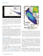
Figure 7. Frequency-transformed distribution of acoustic energy in a typical seismic array pulse such as the one illustrated in Figure 6. Inset (top right): percentage of energy in each frequency band, which can be useful to readers unfamiliar with the logarithmic expressions of pressure and frequency used in acoustics. Note the effects of the “ghost notch” at 125 Hz and multiples thereof. Graphic provided by Schlumberger Ltd.
place the ghost notch at 125 Hz and multiples thereof (250 Hz, 500 Hz, etc.; Figure 7).
Interference between the elements at every angle other than the vertical also affects the total energy and frequency struc- ture of the received sound at different angles around the ar- ray. The lobed sound fields at different frequencies will be familiar to audiometric engineers and acousticians, but for the nonexpert, illustrations of this phenomenon in the hori- zontal plane can be found in BOEM (2014, vol. 3, p. D-15) and in the vertical plane in Goertz et al. (2013, Figure 4).
Sound Propagation
A high level of acoustic energy is needed to image geologi- cal structure at depths of scientific and industrial interest, typically 7 km or more. Energy lost to the water is mini- mal, roughly equal to the spherical spreading of the wave front over a distance equal to the water depth. Even in water depths of 2 km, the loss is small relative to the loss that oc- curs in the rock layers.
The sound that propagates outward in the water pos- es a modeling challenge and is the subject of consider- able ongoing research (e.g., see the Sound and Marine Life Web site: www.soundandmarinelife.org/; also see www.DOSITS.org for a more general discussion of un- derwater sound). Models of the sound field near the
Figure 8. Irregular sound field produced by a seismic airgun array. x- axis: Latitude; y–axis: longitude. Inset: a magnified view of the field above 160 dB SPL, which is too small to see in the larger view. A simi- lar representation of the irregular sound field generated by rectangu- lar arrays of airguns can be found in Goertz et al. (2013). Graphical illustration from MacGillivray (2007), with permission from the Ca- nadian Society of Exploration Geophysicists (CSEG) and the author.
source are well developed and are practical for good pre- dictions of the impulse sound field out to a kilometer or so (Ziolkowski et al., 1982). Models such as Gundalf (Hatton, 2016), Nucleus (Goertz et al., 2013), or AAMS (MacGil- livray, 2006) propagate the impulse in its time-amplitude form, which is computationally complex but gives an accu- rate representation of the pressure wave from which the fre- quency structure can be derived by methods like fast Fourier transform (FFT).
However, propagation over longer distances is done with computationally simpler single-frequency models devel- oped for acoustic oceanography (Medwin and Clay, 1998). For an impulse source such as an airgun, a selected num-
14 | Acoustics Today | Winter 2016