Page 17 - 2016Winter

ber of frequencies are individually modeled and then reas- sembled to generate an estimate of the received sound. Some complexity in the signal is lost in this process and it is not yet clear how significant that loss of accuracy is for assess- ing environmental impacts. The interference patterns of the elements in the array, together with interactions with the environment, do not generate smooth disklike patterns of outward sound propagation. A good illustration of the re- sulting “starlike” pattern of radiated sound can be found in MacGillivray (2007) (Figure 8).
The distinct impulse waveform of 0.1-0.2 s duration near the source is transformed into a series of multiple overlapping and “smeared” arrivals at a distant receiver due to environ- mental interactions en route. The phenomenon, from a sub- jective experiential perspective, is comparable to the sharp “crack” of a nearby lightning strike, compared to the “rum- ble” of distant thunder. These changes to the signal have very real physical and biological implications. Where is the peak amplitude of a signal that now has multiple peaks? What is the total received energy of a signal that may arrive in mul- tiple “packets” over several seconds? What is the perceived “pitch” of the sound when different arrivals have different frequency structures?
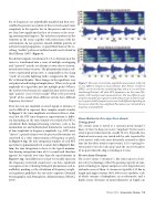
Even for real, not modeled, received signals at distance, it can be difficult to represent these complex sounds visually. In Figure 9, the time-amplitude waveform in blue is iden- tical, but the FFT time-frequency representation is differ- ent depending on the time window over which the FFT is calculated. Both biological hearing structures such as the mammalian ear and mathematical formulas for conversion of time-amplitude to frequency-amplitude (e.g., FFT) must “choose” a period of time over the pressure fluctuations are converted to a static representation of frequency or pitch. In Figure 9, top, the time integration window of each FFT operation is approximately 0.8 seconds, but in Figure 9, bot- tom, the time integration is closer to the typical mamma- lian hearing integration time of 0.2 seconds and therefore appears less smooth over time than the representation in Figure 9, top. Such differences in how we visually represent the frequency-converted sound wave can have significant consequences for evaluating biological phenomena such as audibility, masking, or the calculation of frequency-weight- ed regulatory guidelines for safe noise exposure (National Oceanographic and Atmospheric Administration [NOAA], 2016).
Figure 9. The same received time-amplitude measurement subjected to two different frequency deconvolutions (fast Fourier transform [FFT]): at 0.8-second time windowing (top) and at 0.2-second time windowing (bottom). All other FFT parameters are the same (Mc- Cauley, 2015 and personal communication). The two different ways of representing the same signal reveal that the periods of relative loud- ness or quiet and the frequency structures look different depending on the way in which the time-amplitude fluctuations are translated into frequency and amplitude.
How Seismic Arrays Are Used
Towing Speed
The seismic array is towed at a constant speed around 5 knots (2.5m/s) to keep successive “snapshots” by the source array at precise time intervals, usually 10-20 s. Typically, two identical source arrays are towed side-by-side, separated by a few meters, with each array alternately activated to allow time for the other array to repressurize. A 10-s spacing be- tween pulses (20 s for each array) puts the successive pulses 25 m apart when the ship is traveling at 2.5 m/s.
Receive Array Geometry
The receive arrays (“streamers”), like other aspects of seis- mic survey technology, reflect the growing capacity of com- puter technology to capture and process ever-larger data sets and make sense of them. A streamer is typically 4-12 km in length and might contain 300-1,000 receive modules, each of which contains a hydrophone, an accelerometer, and a depth sensor. Streamers of many kilometers in length can
Winter 2016 | Acoustics Today | 15